Test for Equality of Means (Known Standard Deviation)

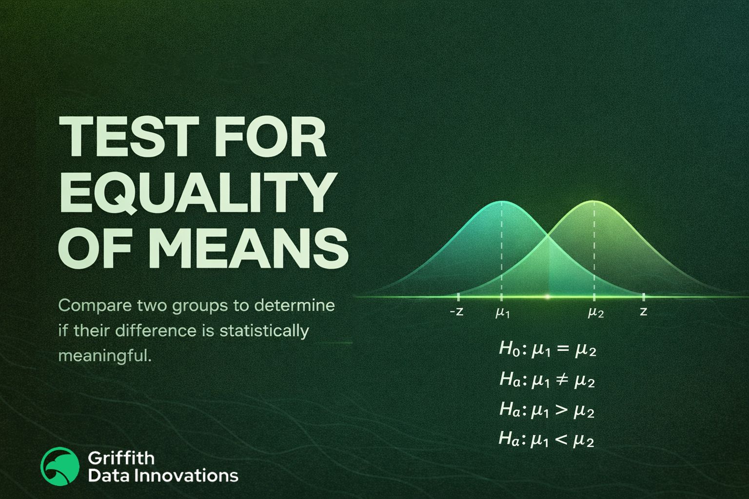
As your analysis becomes more decision-oriented, you will often move beyond evaluating a single average and begin comparing two groups. In business settings, this usually means asking whether a difference in performance, cost, time, or output is statistically meaningful. The test for equality of means with known standard deviations provides a structured way to answer that question when population variability is known.

This test builds directly on the test for one mean. The logic is the same, but now you are comparing two population means instead of one.

What Does “Test for Equality of Means” Mean?

A test for equality of means examines whether two population averages are statistically different from each other.

• In notation, the null hypothesis is written as: 𝐻0 : 𝜇1 = 𝜇2

• This is often rewritten in difference form: 𝐻0 : 𝜇1 − 𝜇2 = 0

The alternative hypothesis depends on the business question:

• Two-sided: 𝐻𝑎 : 𝜇1 − 𝜇2 ≠ 0

• Right-tailed: 𝐻𝑎 : 𝜇1 − 𝜇2 > 0

• Left-tailed: 𝐻𝑎 : 𝜇1 − 𝜇2 < 0

The two-sided version asks whether the averages differ in either direction, while one-sided versions test whether one mean is specifically larger or smaller than the other.

When This Test Is Appropriate

This version of the test applies when:

• You are comparing two independent groups.
• The population standard deviations 𝜎1 and 𝜎2 are known.
• The sampling distributions are normal or the sample sizes are large enough for the central limit theorem to apply.

In practice, knowing the true population standard deviation is uncommon. However, this test is important because it establishes the conceptual foundation for more realistic cases where standard deviations are estimated.

You might encounter this framework in large-scale operational systems where historical process variation is well established and treated as fixed.

The Logic Behind the Test

If the two population means are truly equal, then the difference between sample means should be close to zero, aside from random sampling variation.

Let:

• x1 = sample mean from group 1
• x2 = sample mean from group 2

The key quantity is the difference: x1 − x2

Under the null hypothesis, the expected difference is zero.

Because each sample mean has its own variability, the variability of their difference must account for both sources of uncertainty.

The Test Statistic

When population standard deviations are known, the test statistic follows a standard normal distribution. The formula is:

Z = (x1 – x2) – 0𝜎12n1 + 𝜎22n2

Each part has a clear meaning:

• The numerator measures how far the observed difference is from zero.
• The denominator is the standard error of the difference between means.
• The resulting Z-value tells you how many standard errors the observed difference is from zero.

A value near zero suggests little evidence against 𝐻0. A large positive or negative value suggests the difference is unlikely under the assumption of equal means.

Significance Level and Rejection Regions

As with previous tests, you choose a significance level 𝛼 before examining the results.

For a two-sided test:

• The rejection regions lie in both tails of the standard normal distribution.
• A 95% confidence level corresponds to 𝛼 = 0.05.

If the calculated Z-value falls in the rejection region, you reject 𝐻0. Otherwise, you fail to reject it.

You may also use the p-value approach. If the p-value is less than 𝛼, the null hypothesis is rejected.

This mirrors the structure you saw in the one-mean test. The only difference is that the focus is now on comparing two averages.

A Business Example

Suppose a company operates two warehouses and wants to compare their average order processing times.

Historical data provides known population standard deviations:

• 𝜎1 = 6 minutes
• 𝜎2 = 5 minutes

A random sample is taken from each warehouse:

Warehouse 1:

• 𝑛1 = 40
• x1 = 52 minutes

Warehouse 2:

• 𝑛2 = 35
• x2 = 49 minutes

You want to test whether the average processing times differ.

The hypotheses are:

• 𝐻0 : 𝜇1 − 𝜇2 = 0
• 𝐻𝑎 : 𝜇1 − 𝜇2 ≠ 0

After computing the Z-value, suppose you obtain a p-value of 0.03. At 𝛼 = 0.05, you reject the null hypothesis.

From a business standpoint, this suggests a statistically significant difference in processing times between the two warehouses. The next step is managerial rather than mathematical, and that is to identify operational causes and determine whether adjustments are needed.

Connection to Confidence Intervals

The test for equality of means is closely related to constructing a confidence interval for the difference 𝜇1 − 𝜇2. A confidence interval for the difference takes the form:

(x1 – x2) Z𝜎/2𝜎12n1 + 𝜎22n2

If the value zero lies inside the interval, you would fail to reject the null hypothesis in a two-sided test. If zero lies outside the interval, you would reject it.

This reflects the same principle discussed earlier: a confidence interval contains all values of the hypothesized difference for which the null hypothesis would not be rejected.

Interpreting Results Carefully

Rejecting the null hypothesis indicates statistical evidence of a difference, but it does not explain why the difference exists. This difference can be brought about by operational, environmental, or procedural factors.

Remember that failing to reject the null hypothesis does not prove the two means are identical. It simply means the data does not provide strong enough evidence to conclude otherwise.

Statistical significance should always be considered alongside practical importance. A difference of one minute might be statistically significant in a large sample but irrelevant to customers.

Where This Test Fits in the Bigger Framework

The equality-of-means test with known standard deviations is a conceptual stepping stone. It reinforces the logic of comparing averages while assuming full knowledge of population variability.

In real-world data science and business analytics, you will more often encounter the version where standard deviations are unknown. Still, understanding this known-variance case clarifies how sampling variability works and why adjustments are needed when uncertainty increases. By mastering this structure, you strengthen your ability to evaluate performance differences objectively and support decisions with disciplined statistical reasoning.